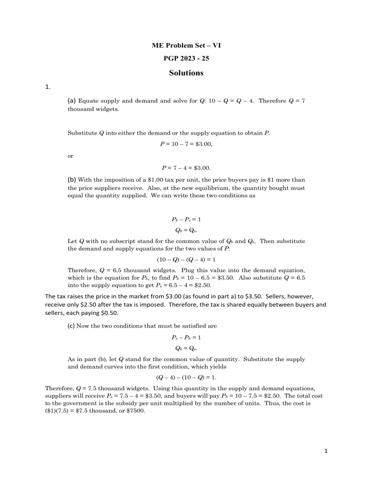
ME Problem Set – VI
PGP 2023 - 25
Solutions
1.
(a) Equate supply and demand and solve for Q: 10 – Q = Q – 4. Therefore Q = 7
thousand widgets.
Substitute Q into either the demand or the supply equation to obtain P.
P = 10 – 7 = $3.00,
or
P = 7 – 4 = $3.00.
(b) With the imposition of a $1.00 tax per unit, the price buyers pay is $1 more than
the price suppliers receive. Also, at the new equilibrium, the quantity bought must
equal the quantity supplied. We can write these two conditions as
Pb – Ps = 1
Qb = Qs.
Let Q with no subscript stand for the common value of Qb and Qs. Then substitute
the demand and supply equations for the two values of P:
(10 – Q) – (Q – 4) = 1
Therefore, Q = 6.5 thousand widgets. Plug this value into the demand equation,
which is the equation for Pb, to find Pb = 10 – 6.5 = $3.50. Also substitute Q = 6.5
into the supply equation to get Ps = 6.5 – 4 = $2.50.
The tax raises the price in the market from $3.00 (as found in part a) to $3.50. Sellers, however,
receive only $2.50 after the tax is imposed. Therefore, the tax is shared equally between buyers and
sellers, each paying $0.50.
(c) Now the two conditions that must be satisfied are
Ps – Pb = 1
Qb = Qs.
As in part (b), let Q stand for the common value of quantity. Substitute the supply
and demand curves into the first condition, which yields
(Q – 4) – (10 – Q) = 1.
Therefore, Q = 7.5 thousand widgets. Using this quantity in the supply and demand equations,
suppliers will receive Ps = 7.5 – 4 = $3.50, and buyers will pay Pb = 10 – 7.5 = $2.50. The total cost
to the government is the subsidy per unit multiplied by the number of units. Thus, the cost is
($1)(7.5) = $7.5 thousand, or $7500.
1
2.
(a) Let the demand curve be of the general linear form Q = a – bP and the supply
curve be Q = c + dP, where a, b, c, and d are positive constants that we have to find
from the information given above. To begin, recall the formula for the price elasticity
of demand
EPD 
P Q
.
Q P
We know the values of the elasticity, P, and Q, so we can solve for the slope, which is
–b in the above formula for the demand curve.
 4.50 
 0 .4  
(  b )
 19.2 
 19.2 
b  0 .4 
  1.71.
 4.50 
To find the constant a, substitute for Q, P, and b in the demand curve formula: 19.2
= a – 1.71(4.50). Solving yields a = 26.9. The equation for demand is therefore Q =
26.9 – 1.71P. To find the supply curve, recall the formula for the elasticity of supply
and follow the same method as above:
E PS 
P Q
Q P
 4.50 
0 .5  
( d )
 19.2 
 19.2 
d  0.5
  2.13
 4.50 
To find the constant c, substitute for Q, P, and d in the supply formula, which yields 19.2 = c +
2.13(4.50). Therefore, c = 9.62, and the equation for the supply curve is Q = 9.62 + 2.13P.
(b) The tax drives a wedge between supply and demand. At the new equilibrium,
the price buyers pay, Pb, will be 40 cents higher than the price sellers receive, Ps.
Also, the quantity buyers demand at Pb must equal the quantity supplied at price
Ps. These two conditions are:
Pb – Ps = 0.40
and
26.9 – 1.71Pb = 9.62 + 2.13Ps.
Solving these simultaneously, Ps = $4.32 and Pb = $4.72. The new quantity will be Q = 26.9 –
1.71(4.72) = 18.8 billion packs. So the price consumers pay will increase from $4.50 to $4.72 and
consumption will fall from 19.2 to 18.8 billion packs per year.
(c) Consumers pay $4.72 – 4.50 = $0.22 and producers pay the remaining $4.50 – 4.32 = $0.18 per
pack.
3. Before the subsidy, the price buyers pay is the same as the price producers receive; call this price
P. The equilibrium can be found by setting supply equal to demand: P/3 =100 – P. Thus, in
equilibrium buyers pay P = $75 / barrel.
In an equilibrium with the subsidy, the price producers receive (Ps) will be $4 per barrel more than
price buyers pay (Pd); thus PS=Pd+4. The market will clear when the quantity bought at a price Pd (i.e.,
100 – Pd) equals the quantity purchased at a price PS = ( i.e., PS/3). Thus, 100 – Pd = PS/3, or 100 – Pd
= (Pd +4)/3. In equilibrium the price paid by buyers is $74, and the price received by producers is $78.
So the reporter’s claim is false; the subsidy reduces the price buyers pay by only $1 per barrel (from
2
$75 to $74 per barrel). The reason that the price does not fall by $4 per barrel is that neither the
demand nor the supply is totally inelastic. Thus the incidence of the subsidy (akin to the incidence of
a tax) is shared by buyers and sellers. The price buyers pay falls by $1, while the price producers
receive rises by $3.
4. a)
Setting Q d  Q s results in
10  P  4  P
P  $7 per bushel
Substituting this result into the demand equation gives Q  3 million bushels.
At the equilibrium, consumer surplus is 1 2 (10  7)3  4.5 and producer surplus is
1 (7  4)3  4.5 . There is no deadweight loss in this case and total net benefits equal $9
2
million.
Price
b)
16.00
14.00
12.00
10.00
8.00
6.00
4.00
2.00
0.00
Supply
Demand
A
B
0
2
4
6
8
10
Quantity (millions of bushels)
In the graph above, area A represents consumer surplus and area B represents producer
surplus.
c)
If the government imposes an excise tax of $2, the new equilibrium will be
10  ( P s  2)  4  P s
P  $6 per bushel
Substituting back into the equation for P d yields P d  8 , and substituting P s into the supply
equation implies Q  2 million.
d)
Now the consumer surplus is 1 2 (10  8)2  2 , the producer surplus is 1 2 (6  4)2  2 ,
the tax receipts are 2(2)  4 , and the deadweight loss is 1 2 (8  6)(3  2)  1 (all measured in
millions of dollars).
3
Price
14.00
12.00
Demand
10.00
A
8.00
C
6.00
B
4.00
2.00
0.00
0
Supply + 2
Supply
D E
2
4
6
Quantity (millions of bushels)
In the graph above, area A represents consumer surplus, area B represents producer surplus,
areas C+D represent government tax receipts, and area E represents the deadweight loss.
e)
If the government provides a subsidy of $1, the new equilibrium will be
10  ( P s  1)  4  P s
P s  $7.5 per bushel
Substituting back into the equation for P d yields P d  6.5 , and substituting P s into the
supply equation implies Q  3.5 million.
Now the consumer surplus is 1 2 (10  6.5)3.5  6.125 , the producer surplus is
1 (7.5  4)3.5  6.125 , the subsidy paid is 1(3.5)  3.5 (negative since the government is
2
paying this amount), and the deadweight loss is 1 2 (7.5  6.5)(3.5  3)  0.25 (all measured in
millions of dollars).
Price
f)
Demand
9.50
8.50
7.50
6.50
5.50
4.50
3.50
2.50
Supply
C
A
B
F
Supply - 1
E
0
0.5
1
1.5
2
2.5
3
D
3.5
4
4.5
5
Quantity (millions of bushels)
In the graph above, areas A+B+E represent consumer surplus, areas B+C+F represent
producer surplus, areas B+C+D+E represent the government subsidy payment, and area D
represents the deadweight loss.
g)
For part (b), the sum of consumer surplus, producer surplus, budgetary impact, and
deadweight loss is 4.5  4.5  0  0  9 ; for part (d), the sum is 2  2  4  1  9 ; and for part (f) it is
4
6.125 + 6.125 – 3.5 + 0.25 = 9. (As above, all are measured in millions of dollars). These sums are all
the same because the deadweight loss measures the difference between net benefits (in terms of
CS, PS, and budgetary impact) under the competitive outcome and net benefits under a form of
government intervention.
5.
(a)
D
S
Equating demand and supply, Q = Q ,
28 – 2P = 4 + 4P, or P = $4.00 per bushel.
To determine the equilibrium quantity, substitute P = 4 into either the supply
equation or the demand equation:
S
Q = 4 + 4(4) = 20 billion bushels,
or
D
Q = 28 – 2(4) = 20 billion bushels.
(b)
Because the free-market supply by farmers is 20 billion bushels, the 25-percent
reduction required by the new Payment-In-Kind (PIK) Program means that the
farmers now produce 15 billion bushels. To encourage farmers to withdraw their
land from cultivation, the government must give them 5 billion bushels of wheat,
which they sell on the market.
Because the total quantity supplied to the market is still 20 billion bushels, the
market price does not change; it remains at $4 per bushel. Farmers gain because
they incur no costs for the 5 billion bushels received from the government. We
can calculate these cost savings by taking the area under the supply curve between
15 and 20 billion bushels. These are the variable costs of producing the last 5
billion bushels that are no longer grown under the PIK Program. To find this
area, first determine the prices when Q = 15 and when Q = 20. These values are
P = $2.75 and P = $4.00. The total cost of producing the last 5 billion bushels is
therefore the area of a trapezoid with a base of 20 – 15 = 5 billion and an average
height of (2.75 + 4.00)/2 = 3.375. The area is 5(3.375) = $16.875 billion.
The PIK program does not affect consumers in the wheat market, because they
purchase the same amount at the same price as they did in the free-market case.
(c) Taxpayers gain because the government does not incur costs to store or destroy the wheat. Although
everyone seems to gain from the PIK program, it can only last while there are government wheat
reserves. The PIK program assumes that the land removed from production may be restored to
production when stockpiles of wheat are exhausted. If this cannot be done, consumers may eventually
pay more for wheat-based products.
5
6.
In this case, the after-subsidy price received by sellers is Ps = Pd + 20. The market-clearing condition
is: 1000 – 10P = 30(P + 20), where P denotes the market price. This implies P = 10 and Q = 900. Since
sellers receive the subsidy, P = Pd = 10 and Ps = Pd + 20 = 30. The surplus implications of the subsidy
are shown below:
With No Subsidy
With Subsidy
Impact of the
Subsidy
A+B
A+B+C+F+G
C+F+G
($28,125)
($40,500)
($12,375)
C+E
C+E+B+I
B+I
($9,375)
($13,500)
($4,125)
Government spending on
subsidy
Zero
B+C+F+G+H+I
-B-C-F-G-H-I
($18,000)
(-$18,000)
Net benefits (consumer
surplus + producer
surplus – government
spending)
A+B+C+E
A+B+C+E-H
-H
($37,500)
($36,000)
(-$1,500)
Deadweight loss
Zero
H ($1,500)
H ($1,500)
Consumer surplus
Producer surplus
P
100
A
S
30
25
C
10
I
B
F
G
H
E
S - 20
D
750
900
Q
1,000
6
7. If demand is perfectly inelastic, the demand curve will be a vertical line. The price will
rise by exactly $2 after the tax is imposed and consumers will take on 100% of the tax
burden. Consumer surplus will fall by $2 times the market quantity, which will be the same
as the pre-tax quantity given the vertical demand curve. Government tax receipts will
increase by $2 times the market quantity completely offsetting the reduction in consumer
surplus. Producer surplus will remain the same since consumers have 100% of the burden of
the tax. Thus, since government receipts completely offset the reduction in consumer
surplus, there is nothing lost to society. There is no deadweight loss from an excise tax when
the demand curve is perfectly inelastic.
7